

ION Lab에서 CNN을 활용하여 졸음운전을 분류해보는 프로젝트를 진행해보았다.
운전자의 특징 변화를 측정함으로써 졸음여부를 판단하는 방법으로 CNN 기반 모델이 운전자의 '눈'을 인식하여 졸음운전 여부를 판단하는 프로젝트이다.
최종 목표는 운전자 CCTV나 블랙박스에서 찍힌 운전자의 사진을 보고 YOLO 등의 모델을 사용하여 Object Detection을 써서 졸음운전을 판단해보는 것인데,
현재로서는 일단 캐글에 있는 Drowsiness Detection 데이터셋을 활용하여 운전자의 눈 사진만 보고 감고 있는지, 뜨고 있는지 분류해보는 간단한 이진분류 프로젝트를 소개하겠다.
https://www.kaggle.com/datasets/kutaykutlu/drowsiness-detection/data
Drowsiness Detection
Human eye images, MRL Eye Dataset
www.kaggle.com
이 포스팅에서는, CNN 모델을 활용하여 진행해 본 프로젝트를 정리하고, 다음 포스팅에서 VGG와 ResNet 모델을 정리해보려고 한다.
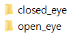
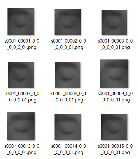
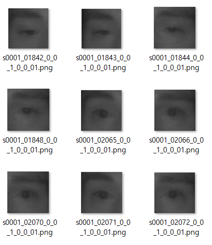
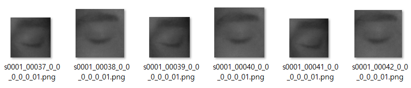
일단 캐글에서 데이터를 다운 받아오면 알아서 눈 감은 사진은 closed_eye에, 눈뜨고 있는 사진은 open_eye 폴더에 저장된다.
- closed_eye
- open_eye
- 데이터 전처리 과정
closed_eye, open_eye에 각각 들어있는 이미지 갯수 확인
import os
folder_path = './data/closed_eye'
files = os.listdir(folder_path)

image_count = 0

for file in files:
    image_count += 1

print('closed_eye 폴더의 이미지 개수 : ', image_count)
closed_eye 폴더의 이미지 개수 : 24000
folder_path = './data/open_eye'
files = os.listdir(folder_path)

image_count = 0

for file in files:
    image_count += 1

print('open_eye 폴더의 이미지 개수 : ', image_count)
open_eye 폴더의 이미지 개수 : 24000

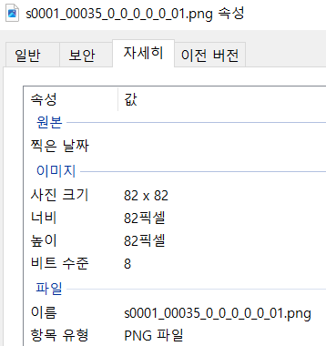
이렇게 각각 이미지 크기가 달랐기 때문에 이미지 크기를 64x64로 통일하고, 텐서로 변환하는 작업을 해줬다.
import torch
from torchvision import datasets, transforms

transform = transforms.Compose([
    transforms.Resize(size = (64,64)), transforms.ToTensor()
])


dataset = datasets.ImageFolder(root='data', transform=transform)
len(dataset)
48000
Q. 사이즈 통일하는 이유
A. CNN은 이미지 공간 구조를 이용하여 특징을 추출하므로 입력 이미지의 크기가 일정하면 네트워크를 설계하고 학습하는 과정이 더 간편해짐. (모든 입력 이미지가 동일한 크기를 가지면 각 레이어의 필터 크기와 풀링 윈도우 크기를 설정하는 것이 훨씬 더 간단해지기 때문)
→ resize를 통해서 이미지 크기 조정하는 건 원본 이미지 파일 자체를 수정하진 않음.
코드에서 이미지를 불러와서 메모리에 임시로 조정한 크기로 변환한 후, 이를 텐서로 변환하여 사용하는 것임. (코드에서 이미지 크기를 조정한 후에 이미지 속성 확인해도 원본 이미지 파일의 크기가 그대로일 것이지만, 이미지가 메모리에 로드될 때는 조정한 크기로 변환되어 있음)
- train, test size 나눠주기
from torch.utils.data import random_split

train_size = int(0.8 * len(dataset))
test_size = len(dataset) - train_size

train_data, test_data = random_split(dataset, [train_size, test_size])

len(train_data), len(test_data)
(38400, 9600)
여기서 DataLoader는 주어진 데이터셋을 미니배치 단위로 효율적으로 로드하여 모델 학습에 활용하기 위한 도구.
train_loader = torch.utils.data.DataLoader(train_data,
                                           batch_size=100, shuffle=True)
test_loader = torch.utils.data.DataLoader(test_data,
                                           batch_size=100, shuffle = False)
이를 통해 데이터를 더 효율적으로 처리하고 학습 속도를 높일 수 있음.
(데이터셋을 여러 개의 미니배치로 분할하고, 각 미니배치에 대해 필요한 전처리를 적용하며, 필요에 따라 데이터를 섞거나 반복적으로 로드하는 등..)
DataLoader 각각 써서 train_loader와 test_loader를 따로 생성하는 것이 일반적임.
Q. train data는 shuffle하고, test data는 주로 shuffle하지 않는 이유?
A. 일반적으로 훈련 데이터셋은 학습이 더욱 효율적으로 이뤄지도록 매 에포크마다 무작위로 섞어줌.
이는 모델이 순서에 의존하지 않고, 다양한 데이터를 보게 해줌으로써 모델의 일반화 성능을 향상시킴. 따라서 보통 훈련 데이터셋은 shuffle함.
↔ 테스트 데이터셋은 모델의 성능을 정확하게 평가하기 위해 사용된 것. 따라서 테스트 데이터셋을 섞으면 모델의 성능을 평가하는 과정에서 데이터의 일관성이 깨질 수 있으며, 모델이 테스트 데이터에 대해 실제로 어떤 성능을 보이는지 정확히 평가할 수 없음.
-label을 각각 숫자 인덱스로 매핑(데이터셋의 클래스 레이블을 숫자인덱스로 매핑)
it = iter(train_loader)
images, labels = next(it)
class_idx = dataset.class_to_idx
print(f"Index of classes are : {class_idx}")
class_names = list(class_idx)
print(f"Class Names are : {class_names}")Index of classes are : {'closed_eye': 0, 'open_eye': 1}
Class Names are : ['closed_eye', 'open_eye']
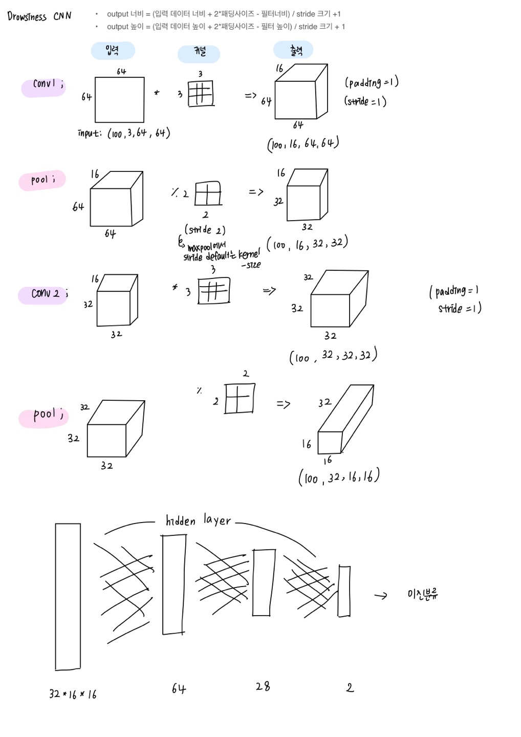
- CNN 모델 생성
class CNNModel(nn.Module):
    def __init__(self):
        super().__init__()

        self.conv_layers = nn.Sequential (
            nn.Conv2d(3, 16, kernel_size=3, stride=1, padding=1),
            nn.LeakyReLU(0.1),
            nn.BatchNorm2d(16),
            nn.MaxPool2d(2),

            nn.Conv2d(16, 32, kernel_size=3, stride=1,padding=1),
            nn.LeakyReLU(0.1),
            nn.BatchNorm2d(32),
            nn.MaxPool2d(2)

        ) #여기서 flatten까지 된 것

        self.linear_layers = nn.Sequential # 또다른 객체를 만들어서 linear layer만 넣음
            nn.Linear(32*16*16, 64),  #여기 사이즈 안맞으면 에러남.
            nn.LeakyReLU(0.1),
            nn.BatchNorm1d(64), # Linear Layer 이므로, BatchNorm1d() 사용해야 함
            nn.Linear(64, 28),
            nn.LeakyReLU(0.1),
            nn.BatchNorm1d(28), # Linear Layer 이므로, BatchNorm1d() 사용해야 함
            nn.Linear(28, 2), # 마지막 출력 뉴런 수 2로 함.
            nn.LogSoftmax(dim=-1)
        )

    def forward(self, x):
        x = self.conv_layers(x) # Conv + Pool
        x = x.view(x.size(0), -1) # Flatten
        x = self.linear_layers(x) # Classification
        return x
- 이진 분류일 때 출력크기
- 보통 마지막 fully connected layer에서 0 또는 1로 분류될 경우에는 마지막 출력 뉴런 수를 1로 하고, 활성화 함수로 시그모이드를 씀 → 손실함수로는 주로 BCE Loss(Binary Cross-Entropy Loss)를 사용함. (실제 클래스가 1인 경우에는 해당 클래스에 대한 예측 확률의 로그 값을, 실제 클래스가 0인 경우에는 반대 클래스에 대한 예측 확률의 로그 값을 계산함. 이를 통해 모델의 예측이 실제 레이블과 얼마나 잘 일치하는지 측정)
- 이진분류를 위해 출력 뉴런의 수가 2가 되는 경우도 있는데, 이런 경우는 일반적으로 하나는 positive, 하나는 negative 클래스에 대한 확률을 나타낼 때 보통 소프트맥스 활성화 함수가 사용되어 두 클래스 간의 확률 값을 정규화함 → 손실함수로 cross-entropy 사용
- 출력 뉴런의 수가 2인 경우에도 로그 소프트맥스 활성화 함수 쓸 수 있는데, 이건 소프트맥스 함수의 로그 변환임. 수치적으로 더 안정적이며, 손실함수로 크로스 엔트로피 손실함수를 사용할 때 수치적으로 더 안정적인 결과 얻을 수 있음.
- 크로스 엔트로피와 비슷하게 사용가능 한 게 Negative Log Likelihood Loss(nn.NLLLoss). 주로 다중 클래스 분류 문제에서 사용되며, 소프트맥스 활성화 함수를 통해 출력된 로그 확률과 실제 클래스 인덱스에 해당하는 로그 확률의 음수 로그 값을 계산하여 모델의 출력이 실제 분포와 얼마나 다른지 측정함.
| 예측 문제 | Regression (숫자 예측, 예 : 키) |
Binary Classification (이진 분류) |
Multi-Class(Multi-Label) Classification (다중 분류) |
| Final Action | None | Sigmoid | Softmax (또는 Log-Softmax) |
| Loss Function | MSE Loss | BCE Loss | Cross Entropy Loss (또는Negative Log Likelihood Loss) |
model1 = CNNModel()
model1
CNNModel(
(conv_layers): Sequential(
(0): Conv2d(3, 16, kernel_size=(3, 3), stride=(1, 1), padding=(1, 1))
(1): LeakyReLU(negative_slope=0.1)
(2): BatchNorm2d(16, eps=1e-05, momentum=0.1, affine=True, track_running_stats=True)
(3): MaxPool2d(kernel_size=2, stride=2, padding=0, dilation=1, ceil_mode=False)
(4): Conv2d(16, 32, kernel_size=(3, 3), stride=(1, 1), padding=(1, 1))
(5): LeakyReLU(negative_slope=0.1)
(6): BatchNorm2d(32, eps=1e-05, momentum=0.1, affine=True, track_running_stats=True)
(7): MaxPool2d(kernel_size=2, stride=2, padding=0, dilation=1, ceil_mode=False)
)
(linear_layers): Sequential(
(0): Linear(in_features=8192, out_features=64, bias=True)
(1): LeakyReLU(negative_slope=0.1)
(2): BatchNorm1d(64, eps=1e-05, momentum=0.1, affine=True, track_running_stats=True)
(3): Linear(in_features=64, out_features=28, bias=True)
(4): LeakyReLU(negative_slope=0.1)
(5): BatchNorm1d(28, eps=1e-05, momentum=0.1, affine=True, track_running_stats=True)
(6): Linear(in_features=28, out_features=2, bias=True)
(7): LogSoftmax(dim=-1)
)
)
- input, output, loss, optimizer 설정
** 주의할 점,
CrossEntropyLoss에는 이미 LogSoftmax가 포함되어 있기 때문에 모델 끝에도 LogSoftmax가 있으면 정확도가 굉장히 낮게 나옴. 문제됨.
→ 모델 내부의 logsoftmax를 빼거나 손실함수를 NLLLoss로 바꿔주면 됨.
device = torch.device("cuda:0" if torch.cuda.is_available() else "cpu")
-train step → train 데이터셋의 loss와 acc 측정
def train_step(model: torch.nn.Module,
               dataloader: torch.utils.data.DataLoader,
               loss_fn: torch.nn.Module,
               optimizer:torch.optim.Optimizer,
               device=device):

    model.train()

    train_loss, train_acc = 0, 0

    for batch, (X,y) in enumerate(dataloader):
        X, y = X.to(device), y.to(device)

        y_pred = model(X)

        loss = loss_fn(y_pred, y)
        train_loss += loss.item()

        optimizer.zero_grad()

        loss.backward()

        optimizer.step()

        y_pred_class = torch.argmax(torch.softmax(y_pred, dim=1), dim=1)
        train_acc += (y_pred_class==y).sum().item()/len(y_pred)

    train_loss = train_loss / len(dataloader)
    train_acc = train_acc / len(dataloader)

    return train_loss, train_acc
-test step → test 데이터셋의 loss와 acc 측정
def test_step(model: torch.nn.Module,
              dataloader: torch.utils.data.DataLoader,
              loss_fn: torch.nn.Module,
              device=device):
    model.eval()

    test_loss, test_acc = 0, 0

    with torch.inference_mode():
        for batch, (X,y) in enumerate(dataloader):
            X, y = X.to(device), y.to(device)

            test_preds = model(X)

            loss = loss_fn(test_preds , y)
            test_loss += loss.item()

            test_pred_labels = test_preds.argmax(dim=1)
            test_acc += ((test_pred_labels == y ).sum().item()/len(test_pred_labels))

    test_loss = test_loss / len(dataloader)
    test_acc = test_acc / len(dataloader)
    return test_loss, test_acc
- 훈련시키기
def training(model: torch.nn.Module,
            train_dataloader,
            test_dataloader,
            optimizer,
            loss_fn: torch.nn.Module = nn.BCELoss(),
            epochs: int = 5,
            device=device):

    results = {"train_loss":[],
               "train_acc":[],
               "test_loss":[],
               "test_acc":[]}
    for epoch in tqdm(range(epochs)):
        train_loss, train_acc = train_step(model=model,
                                           dataloader=train_dataloader,
                                           loss_fn=loss_fn,
                                           optimizer=optimizer,
                                           device=device)
        test_loss, test_acc = test_step(model=model,
                                        dataloader=test_dataloader,
                                        loss_fn=loss_fn,
                                        device=device)

        print(f"Epoch: {epoch} | Train loss: {train_loss:.4f} | Train acc: {train_acc:.4f} | Test loss: {test_loss:.4f} | Test acc: {test_acc:.4f}")

        results["train_loss"].append(train_loss)
        results["train_acc"].append(train_acc)
        results["test_loss"].append(test_loss)
        results["test_acc"].append(test_acc)

    return results
from timeit import default_timer as timer
from tqdm import tqdm
EPOCHS = 5
loss_func = nn.NLLLoss() #negative log likelihood 사용
optimizer = torch.optim.SGD(model1.parameters(), lr=0.01)
start_time = timer()
model1_res = training(model=model1,
train_dataloader=train_loader,
test_dataloader=test_loader,
optimizer=optimizer,
loss_fn=loss_func,
epochs=EPOCHS)
end_time = timer()
print(f"Total training time: {end_time-start_time:.3f} seconds")20%|████████████████▌ | 1/5 [04:23<17:33, 263.39s/it]
Epoch: 0 | Train loss: 0.1285 | Train acc: 0.9568 | Test loss: 0.0736 | **Test acc: 0.9756**
40%|█████████████████████████████████▏ | 2/5 [08:46<13:09, 263.19s/it]
Epoch: 1 | Train loss: 0.0594 | Train acc: 0.9819 | Test loss: 0.0887 | **Test acc: 0.9750**
60%|█████████████████████████████████████████████████▊ | 3/5 [13:22<08:58, 269.18s/it]
Epoch: 2 | Train loss: 0.0435 | Train acc: 0.9865 | Test loss: 0.0644 | **Test acc: 0.9802**
80%|██████████████████████████████████████████████████████████████████▍ | 4/5 [18:30<04:44, 284.53s/it]
Epoch: 3 | Train loss: 0.0345 | Train acc: 0.9900 | Test loss: 0.0452 | **Test acc: 0.9855**
100%|███████████████████████████████████████████████████████████████████████████████████| 5/5 [22:28<00:00, 269.67s/it]
Epoch: 4 | Train loss: 0.0278 | Train acc: 0.9917 | Test loss: 0.0424 | **Test acc: 0.9853** Total training time: 1348.396 seconds
아주 높은 정확도를 보이고 있음 !
- loss와 accuracy 시각화
from typing import Dict, List, Tuple

def plot_loss_curves(results: Dict[str, List[float]]):

    """Plots training curves of a results dictionary."""
    # Get the loss values of the results dictionary(training and test)
    loss = results["train_loss"]
    test_loss = results["test_loss"]

    # Get the accuracy values of the results dictionary (training and test)
    accuracy = results["train_acc"]
    test_accuracy = results["test_acc"]

    # Figure out how mnay epochs there were
    epochs = range(len(results["train_loss"]))

    # Setup a plot
    plt.figure(figsize=(15, 7))

    # Plot the loss
    plt.subplot(1, 2, 1)
    plt.plot(epochs, loss, label="train_loss")
    plt.plot(epochs, test_loss, label="test_loss")
    plt.title("Loss")
    plt.xlabel("Epochs")
    plt.legend()

    # Plot the accuracy
    plt.subplot(1, 2, 2)
    plt.plot(epochs, accuracy, label="train_accuracy")
    plt.plot(epochs, test_accuracy, label="test_accuracy")
    plt.title("Accuracy")
    plt.xlabel("Epochs")
    plt.legend();
import matplotlib.pyplot as plt
plot_loss_curves(model1_res)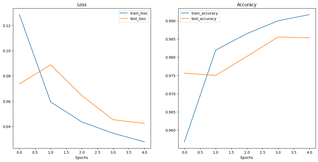
→ 마지막 epoch에서 train 성능은 올라갔는데 test 성능은 떨어짐. 살짝 과적합 되는 경향 보임.
import torch
from sklearn.metrics import confusion_matrix, classification_report

# 모델 평가 모드로 설정
model1.eval()

# 예측값과 실제 레이블을 저장할 리스트 초기화
all_predictions = []
all_labels = []

# 테스트 데이터에 대한 예측 수행
for images, labels in test_loader:
    # 모델이 출력하는 확률 예측
    with torch.no_grad():
        outputs = model1(images)

    # 확률을 클래스 레이블로 변환
    _, predicted = torch.max(outputs, 1)

    # 예측값과 실제 레이블을 리스트에 추가
    all_predictions.extend(predicted.tolist())
    all_labels.extend(labels.tolist())

# Confusion Matrix 계산
cm = confusion_matrix(all_labels, all_predictions)

# Confusion Matrix 출력
print("Confusion Matrix:")
print(cm)

# Classification Report 출력
print("Classification Report:")
print(classification_report(all_labels, all_predictions))
Confusion Matrix:
[[4780 29]
[ 112 4679]]
Classification Report:
precision recall f1-score support
0 0.98 0.99 0.99 4809
1 0.99 0.98 0.99 4791
accuracy 0.99 9600
macro avg 0.99 0.99 0.99 9600
weighted avg 0.99 0.99 0.99 9600
실제로 눈 감았는데, 감았다고 잘 예측한 거 4780
실제로 눈 감았는데, 떴다고 잘못 예측한거 29
실제로 눈 떴는데, 감았다고 잘못 예측한거 112
실제로 눈 떴는데, 떴다고 잘 예측한거 4679
클래스 0에 대한 precision : 0.98 - 눈 감고 있다고 예측한 샘플 중에서 실제로 눈 감고 있는 샘플의 비율.
클래스 0에 대한 recall : 0.99 - 실제로 눈 감고 있는 샘플 중에서 모델이 눈 감고 있다고 정확히 예측한 샘플의 비율
클래스 1에 대한 precision : 0.99 - 눈 뜨고 있다고 예측한 샘플 중에서 실제로 눈 뜨고 있는 샘플의 비율.
클래스 1에 대한 recall : 0.98 - 실제로 눈 뜨고 있는 샘플 중에서 모델이 눈 뜨고 있다고 정확히 예측한 샘플의 비율
위험한 오류→ 눈 감았는데, 떴다고 잘못 예측한거 (졸음운전 중인데, 정상이라고 예측한거니까)
여기서 이 값은 다행히 29으로 제일 낮음. 좋은 모델 !
++ torch. max에 대해서.. torch.max 함수는 주어진 텐서에서 최댓값을 찾아주는 함수임. 보통 분류 문제에서 모델의 출력은 각 클래스에 대한 확률이나 점수로 이루어진 벡터임. 예를 들어 [0.1, 0.8, 0.3]같은 벡터가 있을 때, 이는 각 클래스에 대한 예측 확률을 나타냄. 이 경우 두 번째 클래스가 가장 높은 확률을 갖고 있으므로, 모델의 예측은 두 번째 클래스일 것.
torch.max 함수는 이 중 최댓값을 찾아주며, 첫번재 반환 값으로 최댓값을, 두번째 반환 값으로 최댓값의 인덱스를 반환함. 따라서, "_, predicted = torch.max(outputs, 1)" 여기서는 모델의 출력 outputs에서 각 샘플별로 최댓값과 해당 최댓값의 인덱스를 찾아서 predicted 변수에 저장함. 여기서 두번재 반환 값은 해당 샘플에 대한 예측된 클래스의 인덱스가 됨.
일반 CNN 모델로도 아주 좋은 정확도를 보이고 있다.
다음 포스팅에서는 VGG 모델에 대한 설명과 이를 이용해서 졸음운전을 분류해보는 프로젝트를 정리해보겠다!
'Deep Learning & AI > CV' 카테고리의 다른 글
| [ResNet] 졸음운전 분류 프로젝트 (1) | 2024.03.18 |
|---|---|
| [VGG] 졸음운전 분류 프로젝트 (4) | 2024.03.11 |
| [CNN] 전이 학습 - 특성 추출 기법 (1) | 2024.01.01 |
| [CNN] Fashion MNIST 데이터로 CNN 실습하기 (1) | 2023.12.29 |
| [CNN] Convolutional Neural Network (1) | 2023.12.29 |